Example: detecting defaults on retail credits

SkopeRules finds logical rules with high precision and fuse them. Finding good rules is done by fitting classification and regression trees to sub-samples. A fitted tree defines a set of rules (each tree node defines a rule); rules are then tested out of the bag, and the ones with higher precision are kept.

This example aims at finding logical rules to predict credit defaults. The analysis shows that setting.

Data import and preparation

There are 3 categorical variables (SEX, EDUCATION and MARRIAGE) and 20 numerical variables. The target (credit defaults) is transformed in a binary variable with integers 0 (no default) and 1 (default). From the 30000 credits, 50% are used for training and 50% are used for testing. The target is unbalanced with a 22%/78% ratio.

import numpy as np
import pandas as pd
import matplotlib.pyplot as plt
from sklearn.metrics import roc_curve, precision_recall_curve
from sklearn.ensemble import RandomForestClassifier
from sklearn.model_selection import GridSearchCV
from sklearn.utils import shuffle
from skrules import SkopeRules
from skrules.datasets import load_credit_data

print(__doc__)

rng = np.random.RandomState(1)

# Importing data
dataset = load_credit_data()
X = dataset.data
y = dataset.target
# Shuffling data, preparing target and variables
data, y = shuffle(np.array(X), y, random_state=rng)
data = pd.DataFrame(data, columns=X.columns)

for col in ['ID']:
    del data[col]

# Quick feature engineering
data = data.rename(columns={"PAY_0": "PAY_1"})
old_PAY = ['PAY_3', 'PAY_4', 'PAY_5', 'PAY_6']
data['PAY_old_mean'] = data[old_PAY].apply(lambda x: np.mean(x), axis=1)

old_BILL_AMT = ['BILL_AMT3', 'BILL_AMT4', 'BILL_AMT5', 'BILL_AMT6']
data['BILL_AMT_old_mean'] = data[old_BILL_AMT].apply(
    lambda x: np.mean(x), axis=1)
data['BILL_AMT_old_std'] = data[old_BILL_AMT].apply(
    lambda x: np.std(x),
    axis=1)

old_PAY_AMT = ['PAY_AMT3', 'PAY_AMT4', 'PAY_AMT5', 'PAY_AMT6']
data['PAY_AMT_old_mean'] = data[old_PAY_AMT].apply(
    lambda x: np.mean(x), axis=1)
data['PAY_AMT_old_std'] = data[old_PAY_AMT].apply(
    lambda x: np.std(x), axis=1)

data.drop(old_PAY_AMT + old_BILL_AMT + old_PAY, axis=1, inplace=True)

# Creating the train/test split
feature_names = list(data.columns)
print("List of variables used to train models : " + str(feature_names))
data = data.values
n_samples = data.shape[0]
n_samples_train = int(n_samples / 2)
y_train = y[:n_samples_train]
y_test = y[n_samples_train:]
X_train = data[:n_samples_train]
X_test = data[n_samples_train:]

Out:

List of variables used to train models : [u'LIMIT_BAL', u'SEX', u'EDUCATION', u'MARRIAGE', u'AGE', 'PAY_1', u'PAY_2', u'BILL_AMT1', u'BILL_AMT2', u'PAY_AMT1', u'PAY_AMT2', 'PAY_old_mean', 'BILL_AMT_old_mean', 'BILL_AMT_old_std', 'PAY_AMT_old_mean', 'PAY_AMT_old_std']

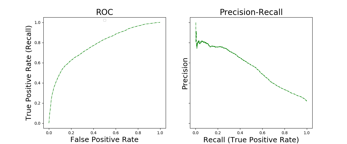
Benchmark with a Random Forest classifier

This part shows the training and performance evaluation of a random forest model. The objective remains to extract rules which targets credit defaults.

rf = GridSearchCV(
    RandomForestClassifier(
        random_state=rng,
        n_estimators=50,
        class_weight='balanced'),
    param_grid={'max_depth': range(3, 8, 1),
                'max_features': np.linspace(0.1, 1., 5)},
    scoring={'AUC': 'roc_auc'}, cv=5,
    refit='AUC', n_jobs=-1)

rf.fit(X_train, y_train)
scoring_rf = rf.predict_proba(X_test)[:, 1]

print("Random Forest selected parameters : %s" % rf.best_params_)

# Plot ROC and PR curves

fig, axes = plt.subplots(1, 2, figsize=(12, 5),
                         sharex=True, sharey=True)

ax = axes[0]
fpr_RF, tpr_RF, _ = roc_curve(y_test, scoring_rf)
ax.step(fpr_RF, tpr_RF, linestyle='-.', c='g', lw=1, where='post')
ax.set_title("ROC", fontsize=20)
ax.legend(loc='upper center', fontsize=8)
ax.set_xlabel('False Positive Rate', fontsize=18)
ax.set_ylabel('True Positive Rate (Recall)', fontsize=18)

ax = axes[1]
precision_RF, recall_RF, _ = precision_recall_curve(y_test, scoring_rf)
ax.step(recall_RF, precision_RF, linestyle='-.', c='g', lw=1, where='post')
ax.set_title("Precision-Recall", fontsize=20)
ax.set_xlabel('Recall (True Positive Rate)', fontsize=18)
ax.set_ylabel('Precision', fontsize=18)
plt.show()

Out:

Random Forest selected parameters : {'max_features': 0.55, 'max_depth': 7}

The ROC and Precision-Recall curves illustrate the performance of Random Forests in this classification task. Suppose now that we add an interpretability contraint to this setting: Typically, we want to express our model in terms of logical rules detecting defaults. A random forest could be expressed in term of weighted sum of rules, but 1) such a large weighted sum, is hardly interpretable and 2) simplifying it by removing rules/weights is not easy, as optimality is targeted by the ensemble of weighted rules, not by each rule. In the following section, we show how SkopeRules can be used to produce a number of rules, each seeking for high precision on a potentially small area of detection (low recall).

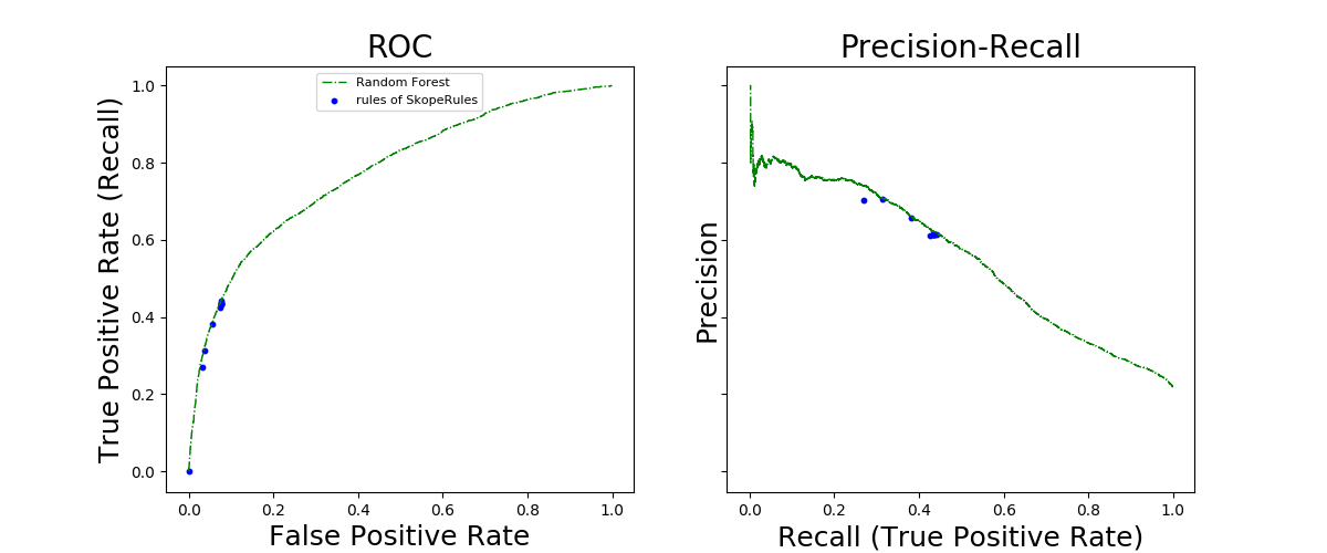
Getting rules with skrules

This part shows how SkopeRules can be fitted to detect credit defaults. Performances are compared with the random forest model previously trained.

# fit the model

clf = SkopeRules(
    max_depth_duplication=3, max_depth=3, max_features=0.5,
    max_samples_features=0.5, random_state=rng, n_estimators=20,
    feature_names=feature_names, recall_min=0.04, precision_min=0.6)
clf.fit(X_train, y_train)

# in the score_top_rules method, a score of k means that rule number k
# vote positively, but not rules 1, ..., k-1. It will allow us to plot
# performance of each rule separately on the ROC and PR plots.
scoring = clf.score_top_rules(X_test)

print(str(len(clf.rules_)) + ' rules have been built.')
print('The 5 most precise rules are the following:')
for rule in clf.rules_[:5]:
    print(rule[0])

curves = [roc_curve, precision_recall_curve]
xlabels = ['False Positive Rate', 'Recall (True Positive Rate)']
ylabels = ['True Positive Rate (Recall)', 'Precision']


fig, axes = plt.subplots(1, 2, figsize=(12, 5),
                         sharex=True, sharey=True)

ax = axes[0]
fpr, tpr, _ = roc_curve(y_test, scoring)
fpr_rf, tpr_rf, _ = roc_curve(y_test, scoring_rf)
ax.scatter(fpr[:-1], tpr[:-1], c='b', s=10, label="rules of SkopeRules")
ax.step(fpr_RF, tpr_RF, linestyle='-.', c='g', lw=1, where='post',
        label="Random Forest")
ax.set_title("ROC", fontsize=20)
ax.legend(loc='upper center', fontsize=8)
ax.set_xlabel('False Positive Rate', fontsize=18)
ax.set_ylabel('True Positive Rate (Recall)', fontsize=18)

ax = axes[1]
precision, recall, _ = precision_recall_curve(y_test, scoring)
precision_rf, recall_rf, _ = precision_recall_curve(y_test, scoring_rf)
ax.scatter(recall[1:-1], precision[1:-1], c='b', s=10,
           label="rules of SkopeRules")
ax.step(recall_RF, precision_RF, linestyle='-.', c='g', lw=1, where='post',
        label="Random Forest")
ax.set_title("Precision-Recall", fontsize=20)
ax.set_xlabel('Recall (True Positive Rate)', fontsize=18)
ax.set_ylabel('Precision', fontsize=18)
plt.show()

Out:

12 rules have been built.
The 5 most precise rules are the following:
BILL_AMT2 > 517.5 and PAY_1 > 1.5 and PAY_AMT_old_std <= 2563.13525391
BILL_AMT_old_std <= 9353.94921875 and PAY_1 > 1.5 and PAY_2 > -0.5
PAY_2 > 1.5 and PAY_AMT_old_mean <= 12955.75 and PAY_old_mean > 0.625
BILL_AMT2 > 1870.0 and PAY_2 > 1.5 and PAY_AMT_old_mean <= 2525.375
BILL_AMT1 > 410.0 and PAY_1 > 1.5 and PAY_old_mean > 0.125

The ROC and Precision-Recall curves show the performance of the rules generated by SkopeRules the (the blue points) and the performance of the Random Forest classifier fitted above. Each blue point represents the performance of a set of rules: Starting from the left on the precision-recall cruve, the kth point represents the score associated to the concatenation (union) of the k first rules, etc. Thus, each blue point is associated with an interpretable classifier, which is a combination of a few rules. In terms of performance, each of these interpretable classifiers compare well with Random Forest, while offering complete interpretation. The range of recall and precision can be controlled by the precision_min and recall_min parameters. Here, setting precision_min to 0.6 force the rules to have a limited recall.

Total running time of the script: ( 3 minutes 55.798 seconds)